
Mathematics has an interesting property of connecting different fields through relatively simple transformations. Starting from logistic regression, I’ll explore what happens when we apply basic mathematical operations like discretization and complex plane extensions to its underlying function. By following these transformations, we end up visiting concepts from dynamical systems, chaos theory, and fractals - fields that might seem distant from the classification algorithms that we data scientists know so well.
Logistic Regression
Let’s begin with a recap of logistic regression, a traditional model widely used in classification problems across various fields. It begins with our attempt at modeling the probability of a binary event - we do so using a log-odds ratio that maps the probability to the real line and estimate this log-odds through a linear model. The logistic regression model is defined as:
$$\log\left(\frac{p}{1-p}\right) = \beta_0 + \beta_1x_1 + \beta_2x_2 + \ldots + \beta_nx_n$$
Where $p$ is the probability of the event, $x_i$ are the features, and $\beta_i$ are the coefficients of the model. The left side of the equation is the log-odds ratio, and the right side is the linear model. This can be expressed as:
$$\log\left(\frac{p}{1-p}\right) = \beta^T x$$
Where $\beta$ is the vector of coefficients and $x$ is the vector of features. If we solve for $p$ we get the logistic function (I won’t derive it here, there’s plenty of Medium posts already doing that):
$$ p = \frac{1}{1 + e^{-\beta^T x}} $$
If we abstract away the coefficients and features, we have:
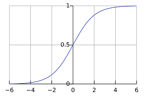
$$ f(x) = \frac{1}{1 + e^{-x}} $$
This is the sigmoid function we all know and love =). It maps the real line to the interval $[0, 1]$, it’s continuous and it’s differentiable. The sigmoid function is also known as the logistic function - this comes from the fact that it’s also the solution of the logistic differential equation.
Logistic Differential Equation
The Logistic Differential Equation models population growth through a simple first-order differential equation. It’s defined as:
$$ \frac{d}{dx}f(x) = r f(x) (1 - f(x)) $$
Where $f(x)$ is the population at time $x$ and $r$ is the growth rate. It is a simple model - population growth is proportional to current size ($rf(x)$) but it’s limited by available resources ($1 - f(x)$). Given the initial condition f(0) = 1/2, the solution of this differential equation is the logistic function.
This basically tells us that, if we get the sigmoid and take its derivative at a given point, the rate of change at that point is proportional to both the current value ($f(x)$) and the remaining value to reach 1 ($1 - f(x)$). This basically gives the typical S-shaped curve, with maximum growth at the middle point and decreasing growth as we reach the limits (both towards 1 and towards 0).
While this differential equation is defined on the real line, we can traverse the mathematical landscape to define the same behavior using discrete rather than continuous values. This brings us to the logistic map…
Logistic Map
The Logistic Map is another model focused on describing population growth and is the discrete version of the logistic differential equation. It describes the population at time $t+1$ as a function of the population at time $t$ and is defined as:
$$ v_{t+1} = r v_t (1 - v_t) $$
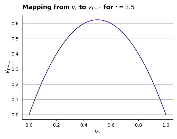
where $v_t$ is the population at time $t$ and $r$ is the growth rate. Unlike the logistic differential equation, this is a discrete model - we’re dealing with distinct time steps rather than continuous time. For a fixed $r$, plotting $v_{t + 1}$ versus $v_t$ yields a simple parabola:
Despite being intuitively a simpler model than a continuously-defined differential equation, it exhibits a very interesting behavior - it is chaotic! The logistic map simulation is straightforward: we set a starting value $v_0$, a growth rate $r$, and iterate the equation. The chart below demonstrates the behavior when starting at $v_0 = 0.5$ and performing 100 iterations for different values of $r$:
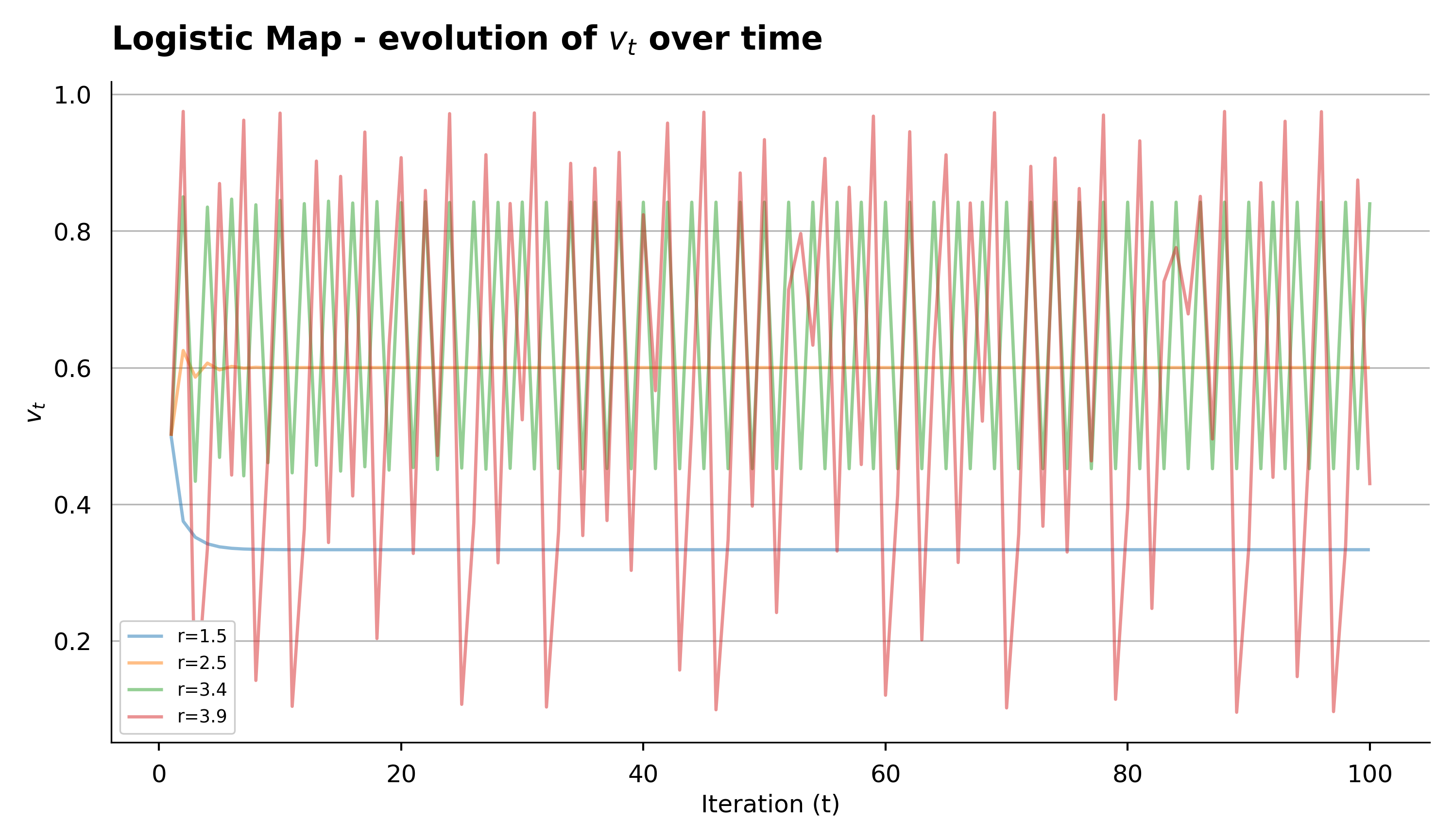
Just by looking at the chart we can see that the behavior is very different for different values of $r$. For $r = 1.5$ and $r = 2.5$ the population converges to a single value, for $r = 3.4$ the population oscillates between two values, and for $r = 3.9$ the population oscillates between four values. This is not a coincidence - the behavior of the logistic map has been widely studied within the realm of chaos theory and it’s chaotic properties are well known!
In fact, for a given value of $v_0$ and $r$ we can actually attribute a numeric value to the infinite sequence of values that the population will take, and can be measured through a concept called Lyapunov exponent. But, we can also visualize this chaotic behavior in a bifurcation diagram.
Bifurcation Diagram
The concept of the bifurcation diagram is elegantly simple: we plot different values of $r$ on the x-axis and the corresponding population values that emerge after many iterations on the y-axis. For each value of $r$, we apply the logistic map repeatedly and identify the values that the population converges to, oscillates between, or diverges to. The result is a fascinating chart that reveals the chaotic behavior of the logistic map, which I show alongside the Lyapunov exponent for each value of $r$:
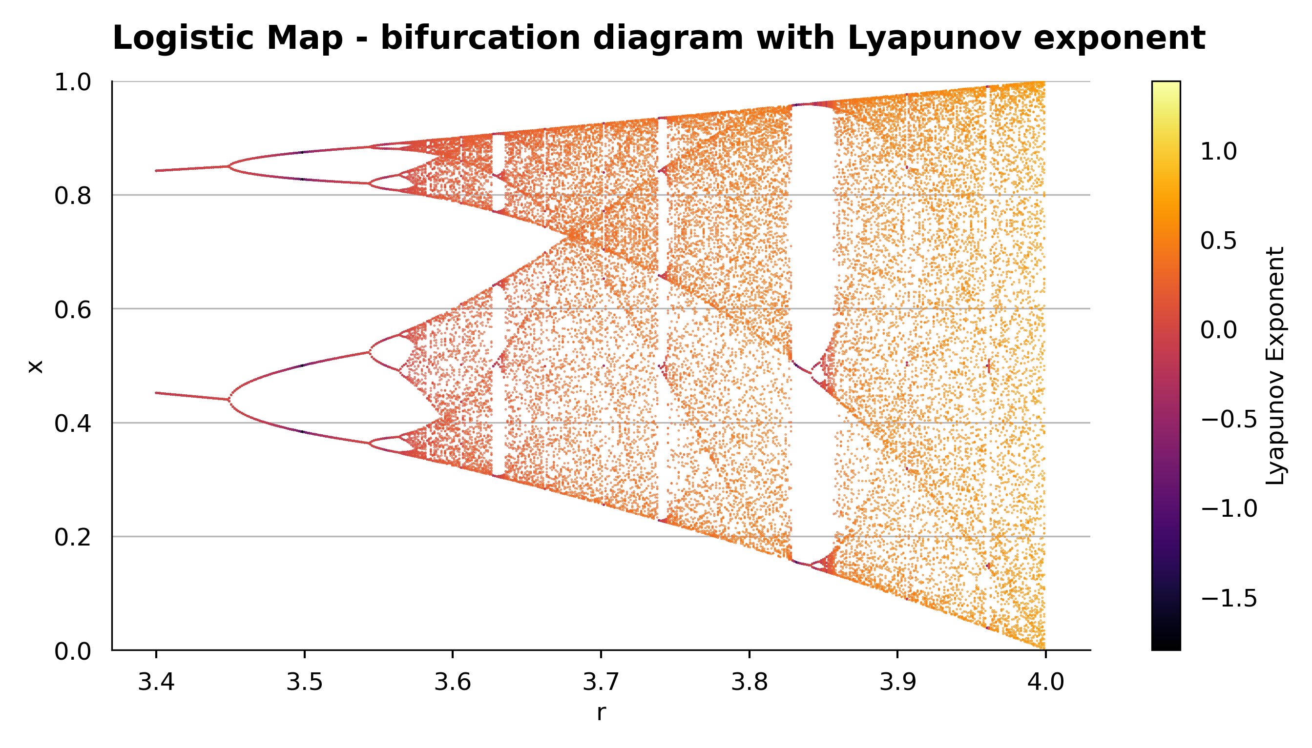
This is a famous visualization in mathematics - it reveals a fractal structure that is common in chaotic systems. The bifurcation diagram is a simple way to visualize the chaotic behavior of the logistic map, and it demonstrates how complex behavior can emerge from a simple model.
Now, we went from the continuous differential equation to the discrete version and we witness the birth of chaos in the system. Now, let’s take a step further and introduce chaos in a more complex space, but still using the same underlying principles.
Chaos in Complex Space
Through scaling and substitutions operations - but preserving the core structure of the logistic map - we can transform the logistic map into a very interesting model. For reference, I’ll add one of the possible derivations of this transformation below:
Starting with the logistic map:
$$ \begin{equation} v_{t+1} = r v_t (1 - v_t) \end{equation} $$
This equation contains a quadratic term $v_t^2$ and a linear term $v_t$ (as we saw in the parabola plotted earlier). The interesting dynamics emerge when these terms balance each other. We know from the sigmoid function that the maximum of $rv_t(1-v_t)$ occurs at $v_t = 1/2$.
This suggests $v_t = 1/2$ as a natural center point for our dynamics. Let’s introduce a change of variables centered around this point:
$$v_t = \frac{z_t + 1}{2}$$
This transformation means:
- When $z_t = -1$, $v_t = 0$
- When $z_t = 0$, $v_t = 1/2$ (center point)
- When $z_t = 1$, $v_t = 1$
The Derivation
Substituting the change of variables:
$$\frac{z_{t+1} + 1}{2} = r(\frac{z_t + 1}{2})(1 - \frac{z_t + 1}{2})$$
Simplify the right side:
$$\frac{z_{t+1} + 1}{2} = r(\frac{z_t + 1}{2})(\frac{1}{2} - \frac{z_t}{2})$$ $$\frac{z_{t+1} + 1}{2} = r(\frac{1}{4} - \frac{z_t^2}{4})$$
Multiply both sides by 2:
$$z_{t+1} + 1 = r(\frac{1}{2} - \frac{z_t^2}{2})$$
Solve for $z_{t+1}$:
$$z_{t+1} = -\frac{r}{2}z_t^2 + \frac{r}{2} - 1$$
If we make a further substitution with $w_t = \sqrt{\frac{r}{2}}z_t$, thus $z_t = \sqrt{\frac{2}{r}}w_t$:
$$\sqrt{\frac{2}{r}}w_{t+1} = -\frac{r}{2}(\sqrt{\frac{2}{r}}w_t)^2 + (\frac{r}{2} - 1)$$
Simplify the right side:
$$\sqrt{\frac{2}{r}}w_{t+1} = -\frac{r}{2}\frac{2}{r}w_t^2 + (\frac{r}{2} - 1)$$ $$\sqrt{\frac{2}{r}}w_{t+1} = -w_t^2 + (\frac{r}{2} - 1)$$
Multiply both sides by $\sqrt{\frac{r}{2}}$:
$$w_{t+1} = -\sqrt{\frac{r}{2}}w_t^2 + \sqrt{\frac{r}{2}}(\frac{r}{2} - 1)$$
we finally get to this final formulation:
$$w_{t+1} = w_t^2 + c$$
where $c = \sqrt{\frac{r}{2}}(\frac{r}{2} - 1)$. To finalize, we now allow $c$ and $w_t$ to be complex numbers:
- $c \in \mathbb{C}$
- $w_t \in \mathbb{C}$
The Mandelbrot Set
The equation we derived generates the famous Mandelbrot set - one of mathematics’ most fascinating objects. We create this fractal by iterating our equation for different values of $c$ in the complex plane, just as we did with the logistic map.

This is one of the most famous mathematical concepts and it’s widely studied in the field of dynamical systems. To finally close the loop, we can also visualize the bifurcation diagram within the Mandelbrot set - a fascinating demonstration of how the chaotic behavior of the logistic map translates into complex space:

Gif by By Jonny Hyman - Own work, CC BY-SA 4.0, https://commons.wikimedia.org/w/index.php?curid=86422564.
Conclusion
What we’ve explored here isn’t just a progression of mathematical complexity, but rather how a series of well-defined mathematical transformations – discretization, solving differential equations, and extending to complex numbers – can take us from familiar territory to unexpectedly rich mathematical landscapes.
Starting from logistic regression, a daily tool in a data scientist’s arsenal, we made a series of mathematically straightforward steps: we found that its sigmoid function solves a differential equation, discretized that equation to discover the logistic map and its chaos, and through some careful variable substitutions in the complex plane, arrived at the Mandelbrot set. Each transformation revealed new behaviors that weren’t obvious from our starting point, highlighting how simple mathematical steps can take us from the predictable realm of classification to systems where predictability itself becomes an intricate question =).