Useful Nonlinear Models in Python

Context

All models are wrong, but some are useful

In statistics, we say that a regression is linear when it’s linear in the parameters. Fitting linear models is an easy task, we can use the least squares method and obtain the optimal parameters for our model. In Python you can achieve this using a bunch of libraries like scipy, scikit-learn, numpy, statsmodels, etc. However, not all problems can be solved with pure linear models. There are a lot of useful nonlinear models that guarantee useful mathematical properties and are also highly interpretable. Since I tend to recurrently fit these models, t article will serve as a future reference for myself whenever I need to use them in the future, with easy to implement code (in Python).

Now, before we get into the models, it’s important to note the context about why and when would you use these types of models. They’re not necessarily a substitute for your complex (XGBoost, LightGBM, Random Forest, Neural Network, etc.) machine learning model. It’s best to think about these nonlinear models in the context of curve fitting, i.e. you want to model a phenomena using a curve that you can interpret later. So, here are some considerations as to why would you use them:

• Interpretability: If you model an event using curves, your outcome is much more interpretable, since usually the mathematical equation has a meaning to each parameter. Important: this doesn’t mean you lose the power of your complex machine learning model, as you can still use the machine learning model alongside the curve you’re fitting (e.g. segment your data using the model, then fit interpretable curves on each segment). This will help not only the person that built the model in the future but also the business stakeholders. It’s much easier to explain what your model is doing if the output is interpretable.

• Mathematical Properties: Sometimes it’s really important to guarantee some mathematical property on your model output. For example if you’re modelling age x height of some insect it probably make sense that your height prediction should be monotonically increasing as age increases. Describing these phenomena using mathematical equations give you the power to apply this constraint in the modelling phase: You just fit a function that has this monotonic property.

Linear x Nonlinear

It’s important to distinguish that when I say nonlinear I mean nonlinear in the parameters. So, for example, a quadratic equation $y = ax^2 + bx + c$ is linear, because this model is linear in the parameters $a, b, c$. The model might not be linear in $x$, but it can still be linear in the parameters.

To give more clarity about linear and nonlinear models, consider these examples:

$$ \begin{equation} y = \beta_0 + \beta_1 x \end{equation} $$

$$ \begin{equation} y = \beta_0 (1 + \beta_1)^x \end{equation} $$

$$ \begin{equation} y = \ \beta_0\cdot\sin\left(x^{\beta_1}\right)\ +\ \beta_2\cdot\cos\left(e^{x\beta_3}\right)\ +\ \beta_4 \end{equation} $$

Equation $(1)$ is a simple line, and the parameters $\beta_0, \beta_1$ are linear on $y$, so this is an example of a linear model. Equation $(2)$ is what we call an Exponential Growth formula, where usually $\beta_0$ represents the starting point, $x$ is a time measure and $\beta_1$ (usually called $r$) represents the growth rate. In this case we want to obtain the starting point and the growth rate; At first you might think that $(2)$ is nonlinear, however you could manipulate the formula to obtain a linear parameterization:

$$ y = \beta_0 (1 + \beta_1)^x \\\
log(y) = log(\beta_0) + x\cdot log(1 + \beta_1) $$

And then call $y'=log(y)$, $\beta_0’ = log(\beta_0)$, $\beta_1'=log(1 + \beta_1)$, you can re-write the Exponential Growth as:

$$y’ = \beta_0’ + \beta_1’x$$

And fit a OLS (Ordinary Least Squares) using this formula, as this is a linear model (this is called a log-linear model)! Finally, equation $(3)$ is a nonlinear model, as the regression is nonlinear in the parameters $\beta_0, \beta_1, \beta_2, \beta_3, \beta_4$ (I hope so, as I created this equation on the fly - if you find a linear parameterization for this equation please let me know).

In this article I’ll first present the main tools we’ll be using to fit the models, and then explain a series of useful nonlinear models + code + graph of the model for whenever you need to fit such marvelous equations. I also won’t go deeper into each model purpose and usage, as it’s not the point of the article.

Fitting curves in Python

A great portion on this article was based on another blogpost, that was aimed at R users, and used R libraries with ready-made equations and built-in routines to facilitate the life of the data scientist. Even though I use R sometimes, most of the time I’m using Python, so it’s nice to keep my project’s codebase with the minimum amount of distinct programming languages. Sadly, there isn’t easy/widespread libraries in Python that have these models built-in (if you know any, please let me know!), so we’ll have to implement the models and be creative in the curve fitting process when needed, especially when choosing the initial parameters guess.

Besides the holy trinity (Pandas, Matplotlib and Numpy), these are the main libraries we’ll use, for fitting purposes:

• Scipy
• Sympy

We’ll mostly use the optimization procedures from Scipy’s curve_fit. The main parameters we’ll be using are:

• f: The function to call when optimizing, i.e. your model. It must have signature similar to my_fn(x, a, b, c, d, ...), where x is your x and a, b, c, d, ... are other parameters. There are other valid signatures, but let’s start with this simple one.
• jac: Optional. The function that returns the Jacobian of your function f. Sometimes it makes the optimization easier as the optimizer won’t have to numerically approximate the gradient of your function.
• xdata: The x values
• ydata: The y values
• p0: Optional (but highly recommended for nonlinear models). The initial guess for the parameters
• bounds: Optional. Constraints for the possible values of each parameter (useful to control general behavior of the optimization)
• maxfev: Optional. Maximum number of function evaluations (basically, how many iterations).

The curve_fit returns the parameters from the optimization, which is what defines the model.

These models also require a somewhat good mathematical knowledge (basic calculus and functions), so that you know what you’re doing. Finally, I’ll also use extensively the amazing tool Desmos to plot our equations. The full code will be available in a Github repo linked at the end of the article.

Initial Guessing and the Jacobian

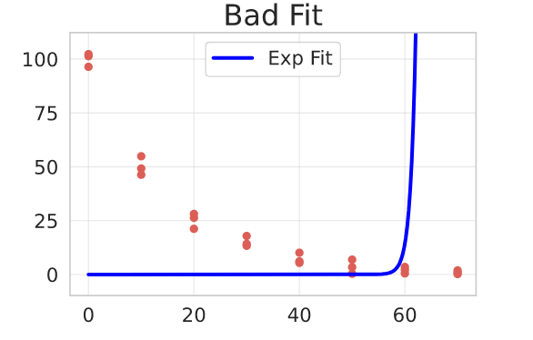
For nonlinear models sometimes it’s crucial that we give the optimizer a good initial guess (p0) for the parameters. Most of the fits I’ll present won’t work without a good guess of their parameters. In R the library drc has built-in routines that helps the user by selecting a good initial configuration of parameters. However I didn’t found something similar in Python, so we’ll have to rely on mathematical intuition and by looking at our dataset. However, I think these routines could be easily implemented, you could write a grid search routine that selects an initial parameter guess and then pass it to curve_fit via the p0 argument (but what’s the fun in that?).

Here’s an example of a bad fit, when you don’t pass the p0 parameter. The model here is an Exponential Decay, presented in the next section and fitted on a chemical reaction substance degradation data. The data is represented in red/pink.

res, pcov = curve_fit(
    f=exponential_model,
    jac=exponential_model_jac, 
    xdata=degradation_df.time,
    ydata=degradation_df.conc,
)

In the snippets below I’ll also provide the Jacobian function for each model. They’re not needed for the fits, as the curve_fit can approximate the gradient of your function numerically, but I’ll present them here for reference (sometimes you might need to take a look at the partial derivatives of your model, you never know). The Jacobian here is simply a column vector with the partial derivatives of your function w.r.t. all of its parameters. I’ll use Sympy to automatically differentiate the expressions, but you could use Wolfram Alpha or the good old pen and paper.

Here’s an example of how to calculate the partial derivatives of a function using Sympy:

from sympy import *
a, b, c, x = symbols("a b c x")
expr = a*x**2 + b*x + c
diff(expr, a), diff(expr, b), diff(expr, c)

$(x^2, x, 1)$

Convex/Concave Models

IMPORTANT: Not all of these models are nonlinear; Some of them can actually be transformed into a linear model - I’m showcasing how one might proceed fitting them directly.

Exponential Decay

Exponential Decay models have a range of different applications for chemistry (substance decay), biology, econometrics, etc.

General parameterisation:

$$Y = a\cdot e^{k\cdot X}$$

Parameters interpretation:

• $a$ is the value of $Y$ when $X = 0$
• $k$ is the relative increase or decrease of $Y$ for a unit increase of $X$

Here we use data on chemical reaction substance degradation, i.e. as time passes the concentration of some substance decreases as it degrades. We want to find the rate the substance degrades overtime. As we saw earlier, if we just pass the function for the curve_fit the result won’t be ideal. So we need to examine our data and our model and provide a good initial guess for the model.

This is why it’s important that you know exactly what you’re trying to model and what the parameters represent! Fit then Predict won’t work =)

From looking at the data and our parameterisation, we can guess that:

• the value of $a$ should be closer to 100
• the value of k should be negative, as the data shows an exponential decay behavior.

Let’s think about k = -1 with a=100. In x=40 the y value would be 100*exp(-40), which results in a very small value (when in fact it should result in something close to 10). So k should be much smaller, for example -1e-3.

Let’s then try the fit with p0=[100, -1e-3] and see what happens:

## functions
def exponential_model(x, a, k):
    return a * np.exp(k * x)

def exponential_model_jac(x, a, k):
    return np.array([np.exp(k * x), a * x * np.exp(k * x)]).T  # transform into column

## fit
res, pcov = curve_fit(
    f=exponential_model,
    jac=exponential_model_jac,
    xdata=degradation_df.time,
    ydata=degradation_df.conc,
    p0=[100, -1e-3],
    bounds=(-np.inf, [np.inf, 0]) # k cannot be greater than 0
)

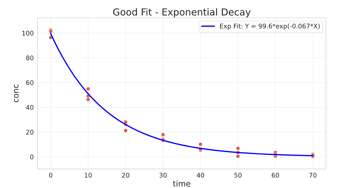
Much better!

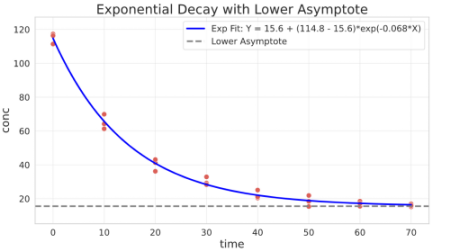
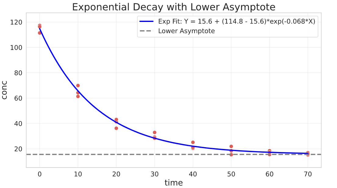
Exponential decay with lower asymptote

General parameterisation:

$$Y = b + (a - b)\cdot e^{k\cdot X}$$

Parameters interpretation:

• $a$ is the value of $Y$ when $X = 0$
• $b$ is the lower asymptote where the decay will stabilize
• $k$ is the relative increase or decrease of $Y$ for a unit increase of $X$

## functions
def exponential_decay_asymptote(x, a, b, k):
    return b + (a - b) * np.exp(k * x)


def exponential_decay_asymptote_jac(x, a, b, k):
    return np.array([np.exp(k * x), 1 - np.exp(k * x), x * (a - b) * np.exp(k * x)]).T


offset = 15  # manual concentration offset for illustration purpose
## fit
res, pcov = curve_fit(
    f=exponential_decay_asymptote,
    jac=exponential_decay_asymptote_jac,
    xdata=degradation_df.time,
    ydata=degradation_df.conc + offset,
    p0=[100, 10, -1e-3],  # putting 10 as a starting point for the lower asymptote
    bounds=(-np.inf, [np.inf, np.inf, 0]),  # k cannot be greater than 0
)
a, b, k = res

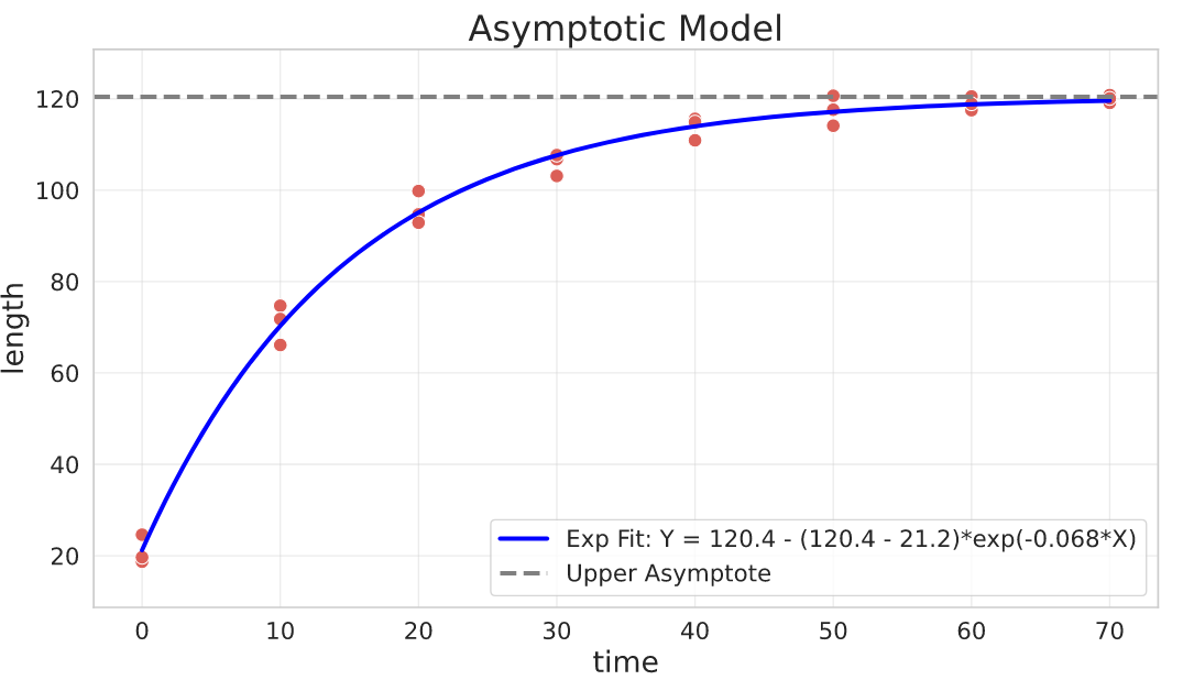
Asymptotic Model (Negative Exponential)

Basically the opposite of the exponential decay model. It can be used to describe phenomena where $Y$ has a limited growth as $X$ goes to infinity.

For example, if $Y$ is the length of a fish and $X$ represents its age, we expect a growth (increase in the fish length) as it ages, but it won’t constantly increase in length, it will probably stabilize on maximum obtainable length. This fish example was based on the von Bertalanffy law. Also, we don’t expect the fish to have $0$ length when it’s born, so the common parameterisation of this type of model also has a parameter to control this.

General parameterisation:

$$Y = b - (b - a)\cdot e^{-k\cdot X}$$

Parameters interpretation:

• $a$ is the value of $Y$ when $X = 0$
• $b$ is the upper asymptote where the growth will stabilize (maximum attainable value for $Y$)
• $k$ is the relative increase or decrease of $Y$ for a unit increase of $X$

## functions
def negative_exponential_asymptote(x, a, b, k):
    return b - (b - a) * np.exp(-k * x)


def negative_exponential_asymptote_jac(x, a, b, k):
    return np.array(
        [np.exp(-k * x), 1 - np.exp(-k * x), -x * (a - b) * np.exp(-k * x)]
    ).T


## fit
res, pcov = curve_fit(
    f=negative_exponential_asymptote,
    jac=negative_exponential_asymptote_jac,
    xdata=growth_data_df.time,
    ydata=growth_data_df.length,
    p0=[
        0,
        200,
        1e-3,
    ],  # Y can start at 0 when X=0, the asymptote guess is 200 and the rate guess is 1e-3
    bounds=(0, [np.inf, np.inf, 1]),  # adding constraints
)
a, b, k = res

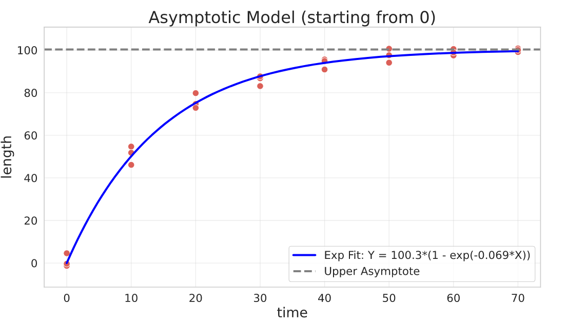
Asymptotic Model (constrained: starting from 0)

Sometimes your model needs to start from 0 (i.e. $a = 0$ from the previous equation). This results in a simpler parameterisation, albeit with the same behavior.

General parameterisation:

$$Y = b\cdot (1 - e^{-k\cdot X})$$

Parameters interpretation:

• $b$ is the upper asymptote where the growth will stabilize (maximum attainable value for $Y$)
• $k$ is the relative increase or decrease of $Y$ for a unit increase of $X$

## functions
def negative_exponential(x, b, k):
    return b * (1 - np.exp(-k * x))


def negative_exponential_jac(x, b, k):
    return np.array([1 - np.exp(-k * x), b * x * np.exp(-k * x)]).T


offset = -20
## fit
res, pcov = curve_fit(
    f=negative_exponential,
    jac=negative_exponential_jac,
    xdata=growth_data_df.time,
    ydata=growth_data_df.length + offset,
    p0=[200, 1e-3],  # the asymptote guess is 200 and the rate guess is 1e-3
    bounds=(0, [np.inf, 3]),  # adding constraints
)
b, k = res

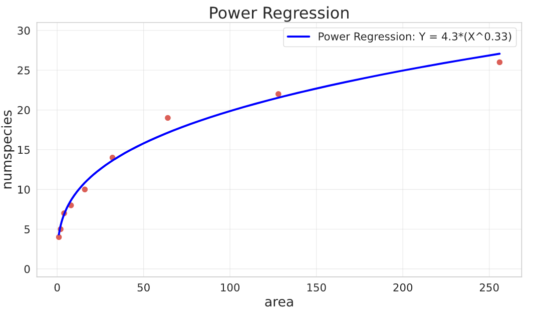
Power Regression

General parameterisation:

$$Y = a\cdot X^{b}$$

Parameters interpretation:

• $a$ is the value of $Y$ when $X = 0$
• $b$ is the power (controls how $Y$ increases relative to $X$

The Power Regression is equivalent to an exponential curve but with the logarithm of $X$:

$$aX^b = a\cdot e^{log(X^b)} = a\cdot e^{b\cdot log(X)}$$

## functions
def power_regr(x, a, b):
    return a * np.power(x, b)


def power_regr_jac(x, a, b):
    return np.array([np.power(x, b), a * np.power(x, b) * np.log(x)]).T


## fit
res, pcov = curve_fit(
    f=power_regr,
    jac=power_regr_jac,
    xdata=species_df.area,
    ydata=species_df.numspecies,
    p0=[200, 2],  # it starts at 0, power guess is 2 (quadratic behavior)
)
a, b = res

Here I’m fitting a Power model to a dataset that has the number of plant species by sampling area of some experiment.

• area: total area of sampled space for measuring the plants
• numspecies: number of species found

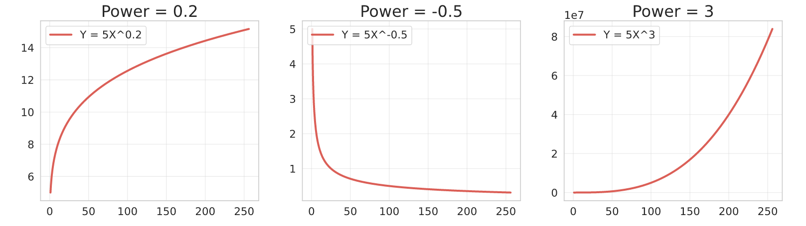
A useful property of the Power parameter is that you can bound it in the fit depending on the growth behavior you’re trying to model.

• $0 < b < 1$: Convex shape, $Y$ increases as $X$ increases.
• $b < 0$: Concave shape, $Y$ decreases as $X$ increases.
• $b > 1$: Concave shape, $Y$ increases as $X$ increases.

Here are some examples:

Sygmoidal Curves

Here are two main curves to test when you need to model events which have a sygmoidal shape.

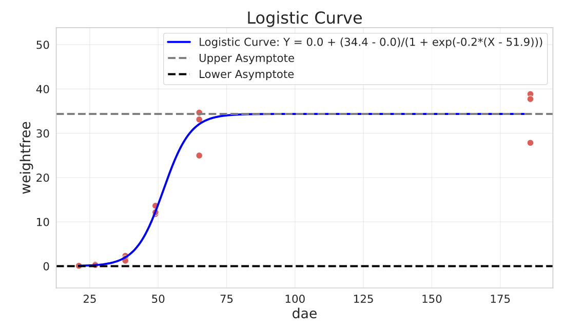
Logistic Curve

The logistic curve should be familiar to any data scientist. It’s derived from the cumulative logistic distribution function and is symmetric around a inflection point.

General parameterisation:

$$Y = a + \frac{c - a}{1 + e^{b(X - d)}}$$

Parameters interpretation:

• $c$ is the upper asymptote
• $a$ is the lower asymptote
• $d$ controls the location of the inflection point (relative to X)
• $b$ the slope around the inflection point, and we can use it to control the ‘growth’ behavior. If $b < 0$, then $Y$ increases as $X$ increases and if $b > 0$ then $Y$ decreases as $X$ increases.

This parameterisation above is general, but depending on what you’re trying to fit it can be reduced. For example, if we se $a = 0$ we have a simpler equation. We could also force $c = 1$ furthermore, making the equation even simpler. It all depends on the constraints of your problem.

def logistic_curve(x, a, b, c, d):
    return a + (c - a) / (1 + np.exp(b * (x - d)))


def logistic_curve_jac(x, a, b, c, d):
    return np.array(
        [
            1 - (1 / (np.exp(b * (-d + x)) + 1)),
            ((-a + c) * (-d + x) * np.exp(b * (-d + x)))
            / (np.exp(b * (-d + x)) + 1) ** 2,
            (1) / (np.exp(b * (-d + x)) + 1),
            (b * (-a + c) * np.exp(b * (-d + x))) / (np.exp(b * (-d + x)) + 1) ** 2,
        ]
    ).T


## fit
res, pcov = curve_fit(
    f=logistic_curve,
    jac=logistic_curve_jac,
    xdata=beetgrowth_df.dae,
    ydata=beetgrowth_df.weightfree,
    p0=[
        0,
        -0.1,
        50,
        30,
    ],  # lower asymptote guess is 0, b is negative (Y increases with X), upper asymptote guess is 50 and inflection point guess is at 30 dae
    bounds=([0, -np.inf, -np.inf, -np.inf], [0.1, 0, np.inf, np.inf]),
    maxfev=3000,
)
a, b, c, d = res

In this example we fit a Logistic Curve to model Plant Growth, in this case Sugar Beet. The variables are:

• dae: days after plant emergence
• weightfree: Weight measurements (grams per square meter of dry matter)

The dataset was published in this paper: Scott, R. K., Wilcockson, S. J., & Moisey, F. R. (1979). The effects of time of weed removal on growth and yield of sugar beet.

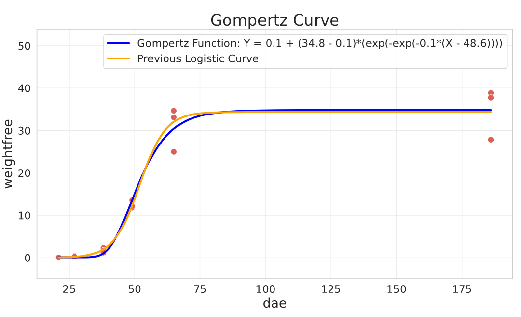
Gompertz Function

Or more specifically, the Gompertz Curve. Not always the problem we’re modelling is symmetric, and the Gompertz function can model different “growth speeds” around the inflection point. I suggest you take a look at the Wikipedia page for this function, here are some examples of where it can be used:

• Mobile phone uptake, where costs were initially high (so uptake was slow), followed by a period of rapid growth, followed by a slowing of uptake as saturation was reached
• Population in a confined space, as birth rates first increase and then slow as resource limits are reached
• Modelling of growth of tumors
• Modelling market impact in finance and aggregated subnational loans dynamic.

General parameterisation:

$$Y = a + (c - a)\cdot e^{-e^{b(X - d)}}$$

The parameters have similar interpretation as in the Logistic Curve.

Parameters interpretation:

• $c$ is the upper asymptote
• $a$ is the lower asymptote
• $d$ controls the location of the inflection point
• $b$ the slope around the inflection point, and we can use it to control the ‘growth’ behavior. If $b < 0$, then $Y$ increases as $X$ increases and if $b > 0$ then $Y$ decreases as $X$ increases.

def gompertz_function(x, a, b, c, d):
    return a + (c - a) * np.exp(-np.exp(b * (x - d)))


def gompertz_function_jac(x, a, b, c, d):
    return np.array(
        [
            1 - np.exp(-np.exp(b * (-d + x))),
            -(-a + c) * (-d + x) * np.exp(b * (-d + x)) * np.exp(-np.exp(b * (-d + x))),
            np.exp(-np.exp(b * (-d + x))),
            b * (-a + c) * np.exp(b * (-d + x) * np.exp(-np.exp(b * (-d + x)))),
        ]
    ).T


## fit
res, pcov = curve_fit(
    f=gompertz_function,
    jac=gompertz_function_jac,
    xdata=beetgrowth_df.dae,
    ydata=beetgrowth_df.weightfree,
    p0=[
        0,
        -0.1,
        50,
        30,
    ],  # lower asymptote guess is 0, b is negative (Y increases with X), upper asymptote guess is 50 and inflection point guess is at 30 dae
    bounds=([0, -np.inf, -np.inf, -np.inf], [0.1, 0, np.inf, np.inf]),
    maxfev=3000,
)
a, b, c, d = res

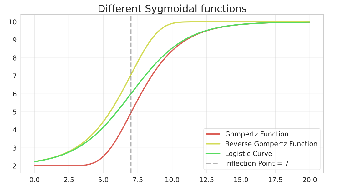
The Gompertz Curve has an alternative parameterisation that inverts the growth pattern from the general one:

$$Y = a + (c - a)\cdot \left[1 - e^{-e^{-b(X - d)}}\right]$$

I won’t fit anything to it as it’s quite similar to the previous one.

Here is an example to better visualize the difference between the sygmoidal curves. The parameters here are: a=2, b=-0.5, c=10, d=7

def reverse_gompertz_function(x, a, b, c, d):
    return a + (c - a) * (1 - np.exp(-np.exp(-b * (x - d))))


a, b, c, d = 2, -0.5, 10, 7

Conclusion + Code

I hope these snippets and code examples will prove useful to you (and to my future self). There are a lot of other nonlinear models that I didn’t include, some of them are:

• Michaelis-Menten equation
• Yield-loss/density curve
• Log-logistic curve
• Weibull curve

As mentioned earlier, this article was based on another article which include more details about the equations above, albeit all the fitting code is in R. Some of the datasets I used were also taken from the aomisc package in R.

Finally, you can find all the code + datasets here in my Github repo.