
Gradient Boosting
GBM or Gradient Boosting Machines are a form of machine learning algorithms based on additive models. The currently most widely known implementations of it are the XGBoost and LightGBM libraries, and they are common choices for modeling supervised learning problems based on structured data. Generally, the output model in boosting is created by iteratively building weak learners, where each new weak learner weights more the mispredictions of the last learner, and so on. Almost all of the current gradient boosting libraries implement these base weak learners as decision trees, and this is one of the reasons for the efficiency of these algorithms.
It can be thought of as a sum of multiple weak learners $F_m$ built on a stagewise fashion, where each $F$ is (in XGBoost and LightGBM) a decision tree. So if the model is trained with $M$ trees, the final model can be interpreted as:
$$ F_M(x) = F_0(x) + \sum_{m=1}^{M}F_m(x)$$
If you’re interested in understanding more about the peculiarities of GBMs or why it usually gives good results, I highly recommend checking the first three chapters of my undergraduate thesis and the paper Why Does XGBoost Win “Every” Machine Learning Competition?. XGBoost and LightGBM both introduced new and smart ways to make the algorithm computationally efficient while keeping approximately the accuracy. This post aims to showcase and give more intuition into one of these improvements, which is using histograms instead of feature values when finding the optimal splits for a given tree node. There are other improvements made as well, like GOSS and EFB (described more in-depth in the LightGBM paper), but I won’t tackle these two for now.
The bottleneck of a decision tree
Let’s focus on the building process of a single tree $F_m$. The induction of decision trees can be seen as a Greedy Algorithm, usually in a top-down approach where at each node of the tree a pair $(f, f_t)$ is chosen. The notation here is that $f$ is a feature and $f_t$ is a threshold value of the said feature. What the node represents can be interpreted as a question:
“is $f < f_t$? if yes continue to the left child, else go to the right child”
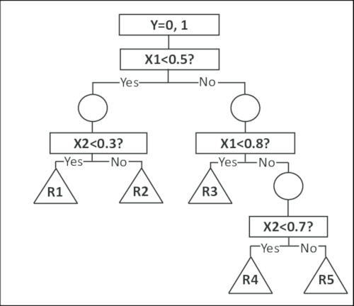
In a decision tree, the objective is to find the best pair $(f, f_t)$ according to a metric of entropy, usually Information Gain or Gini Impurity. So, to put this split finding algorithm in simple terms:
for each feature f:
    for each feature threshold value f_t:
        compute gain if splitting this node using (f, f_t)

choose (f, f_t) with the best gain
In each node of the GBM algorithm, the gain only depends on the sum of gradients of the left child, the right child, and the current node. To calculate these sum of gradients fast, a typical approach is to sort the values of the feature being tested. For example, suppose all unique values of the feature “age” are $[30, 44, 10, 55, 8, 19, 22]$. These values are sorted into $[8, 10, 19, 22, 30, 44, 55]$ and sequentially test increasingly higher values of threshold $f_t$.
One might recall that for sorting algorithms that make comparisons, it isn’t possible to achieve have better complexity than $\mathcal{O}(n\ log\ n)$. So the split finding process complexity can be approximated to $\mathcal{O}(|F|\cdot n\ log\ n)$, where |F| is the number of features that are being evaluated and $n$ the number of values to evaluate for each one of them (they could be different, but for simplicity purposes, I’m assuming they’re the same).
So, could this split finding algorithm be more efficient? 🤔🤔
Histogram to the rescue
This approach can be better understood thinking in terms of splitting continuous features, and the basic idea is to approximate the threshold values using some form of quantization. In LightGBM the algorithm creates a histogram of feature values, with equal bin density (i.e. transforms the feature distribution into a uniform distribution for split finding), built using a subset of the dataset (controlled by the bin_construct_sample_cnt parameter).
Gradient binning
So, here’s an example of how this works and why it improves performance. Consider this training set with just two features $f_1$ and $f_2$, represented in each column:
$$ \left[ \begin{matrix}
1.5 & 0.0\\\
0.0 & 5.5\\\
0.3 & 7.0\\\
5.5 & 8.5
\end{matrix} \right]$$
And then the equal density histogram for each feature is created, replacing each feature value with the index of the bin that value is mapped to! So if the histogram has 3 buckets/bins, this could be the output after the binning procedure:
$$ \left[ \begin{matrix}
1 & 0\\\
0 & 1\\\
0 & 2\\\
2 & 2
\end{matrix} \right]$$
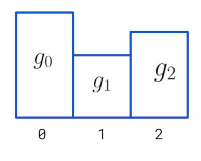
But what information does the histogram have exactly? Recall that to compute the gain it’s only necessary to have the sum of gradients for the left child, the right child, and the current node. So, this sum of gradients is stored in each bin of the histogram, which allows for faster computation of the gain. At first, the algorithm complexity was $\mathcal{O}(n\ log\ n)$, but by using histograms it’s now reduced to $\mathcal{O}(n\_bins)$! In LightGBM $n\_bins=255$ (can be changed with the max_bin parameter), and this is one of the reasons for the huge performance increase of modern gradient boosting frameworks.
Each value maps to the index in the histogram ($g_i$ represent the sum of gradients from data inside bin $i$):
Subtraction trick
This is also a simple yet cool trick used when calculating the gain of a node in this splitting process. The gain function for a node is more complicated as it involves the hessian and regularization parameters, but let’s simplify things a little bit. As assumed earlier, the left and right child gradients are enough to calculate the gain of a node:
$$\sum{g_i} = \sum_{k \in \text{ left}}{g_k} + \sum_{k \in \text{ right}}{g_j}$$
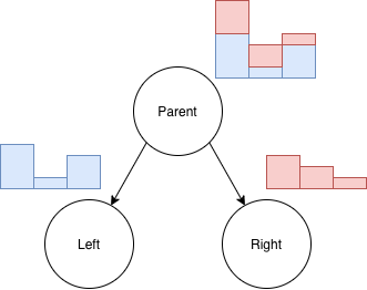
When considering a split value for a feature, the values are either mapped to the left or right child. So, the gradients follow this simple rule that $Histogram(parent) = Histogram(left) + Histogram(right)$, which means it’s possible to calculate the gain/histogram of one of the child nodes and subtract it from the current node (which is already calculated), and the histogram of gradients for the other child is obtained “automatically”.
In practice, this reduces the histogram building process from $\mathcal{O}(n)$ (looking up all the data points in the current node to build the histogram ) to $\mathcal{O}(n\_bins)$ for half the cases due to the subtraction trick, as it isn’t necessary to manually build the histogram for one of the children. Usually the algorithm calculates the histogram for the child with the smallest $n$ and get the other child histogram via the subtraction trick.
The following figure illustrates this: starting with the Parent histogram and calculating the Left histogram (blue), their subtraction results in the red histogram, which corresponds to the Right child histogram!
References
And that’s it! By using an approximate solution the whole training process gradient boosting gets a huge boost👀 in computational performance. This approach is being adopted and added to a lot of different frameworks too, e.g. you can check the code for the subtraction trick in this Cython code for Scikit-Learn, and they even have a similar approach in HistGradientBoostingClassifier and HistGradientBoostingRegressor, inspired by LightGBM!
Finally, the following parameters can be used to alter the default behavior of the histograms in LightGBM (use it carefully):
bin_construct_sample_cntmin_data_in_bindata_random_seedmax_bin
More details about each of them can be found in the LightGBM parameters documentation.